Project Structure and Workflow

Every research project in the lab starts from the same template repository. This appendix explains the reasoning behind that template — why the folders exist, how scripts should communicate, and which conventions keep a project reproducible six months (or six years) after the last commit.

The template README covers what goes where. This appendix covers why and how.

The Project-Oriented Workflow

Every project in the lab lives in one folder. This project folder holds all elements of a project: code, data, manuscripts, figures, etc. The .Rproj file marks that root. All your file paths should be relative to it (i.e., never absolute).

Two rules make this work.

Never use setwd()

Using setwd() hard-codes a path that exists only on your computer. A collaborator who clones your repo hits an error on line 1. The {here} package solves this: here::here("data", "clean.csv") resolves relative to the .Rproj root, regardless of who runs it or where.¹

## Good
raw_df <- readr::read_csv(here::here("data_raw", "acs_2020.csv"))

## Bad — only works on one machine
raw_df <- readr::read_csv("/Users/me/projects/mortality/data_raw/acs_2020.csv")

## Also bad — fragile relative path
raw_df <- readr::read_csv("../../data_raw/acs_2020.csv")

Highly recommended reading. Read Jenny Bryan’s “Project-oriented workflow” post for more details.

Never rely on leftover workspace objects

The .Rproj file in our template ships with three settings that differ from RStudio’s defaults:

Setting	Template value	RStudio default	Why
RestoreWorkspace	No	Yes	A reproducible script runs from a clean environment
SaveWorkspace	No	Ask	Leftover .RData files mask broken code
AlwaysSaveHistory	No	Yes	History files add noise to Git diffs

If your script only works because a previous session left objects in memory, that is a bug. Restart R often using:

• Windows / Linux: Ctrl+Shift+F10
• macOS: Cmd+Shift+F10

Before shipping code or asking a collaborator to run something, hit Cmd+Shift+F10 (or Ctrl+Shift+F10) one last time and confirm everything still works.

Warningrm(list = ls()) is not a substitute

rm(list = ls()) clears the global environment but leaves loaded packages, altered options, and modified search paths intact.

For example, if a previous script ran library(dplyr), then dplyr::filter() still masks stats::filter() after rm(list = ls()) — and any options() you changed (e.g., scipen, stringsAsFactors) remain altered. A full R restart is the only reliable reset. If you see rm(list = ls()) at the top of a script, delete it and test with a fresh session instead.

The Modular Pipeline

Each script in code/ does one job: read some input files, do some work, write some output files. Scripts communicate through files on disk, not objects in memory. For example, a code file may take in (messy) raw data, then save cleaned data in a new folder. The next code then reads in the cleaned data to fit a model. The final code file may read in the model outputs to make plots.

data_raw/ ──→ code/01_clean_data.R   ──→ data/
data/     ──→ code/02_fit_models.R   ──→ output/
output/   ──→ code/03_make_figures.R ──→ plots/

This design has four concrete payoffs:

1. Code review is tractable. A reviewer reads one small script, not one 1,000-line monolith. The reviewer knows what the input and output of that script is, which makes manually checking the work much easier. Once that file has been reviewed, we never need to open it again unless we change something.
2. Intermediate data can be reused. Multiple downstream scripts can read the same cleaned dataset without re-cleaning. Model diagnostics can be run without refitting the models.
3. Expensive steps can be skipped. If 01_clean_data.R takes 30 minutes and the raw data have not changed, it can be skipped.
4. Pipeline managers are portable. Tools like {targets} or make slot naturally onto a pipeline of numbered scripts. A monolithic script gives them nothing to work with.

The key principle is that every script’s inputs and outputs are explicit, named, and written to disk. “It only works if you run this other script first and don’t restart R” is not a pipeline — it’s a trap.

NoteNon-linear pipelines are fine

Real projects are rarely perfectly linear. 01_clean.R might feed both 02_fit_models.R and 03_descriptive_stats.R. That’s fine — the numbering reflects approximate execution order, not a strict chain. What matters is that each script’s ## Input: / ## Output: header makes the dependency structure explicit so a collaborator can see which scripts can run independently.

TipWhen to break a script in two

In general, a script should do one thing really well so that when we review that code and know it works, we don’t need to check it again. If a script is complex, outputting multiple files, or is excessively long, it should (when possible) be broken into smaller scripts.

As a rough heuristic: if a script exceeds ~200–300 lines of non-comment code, or if you find yourself adding section headers for conceptually unrelated tasks (e.g., “clean data” and “fit models” in the same file), it’s time to split. Note that this is a very rough rule of thumb — counting lines of code is a poor metric. Code with lots of lines but just one conceptual objective (that cannot be broken up) should stay in a single file.

Naming Conventions

Scripts

Scripts follow a NN_verb_slug.R pattern. The zero-padded prefix sets execution order. The verb-slug describes what the script does.

Do this

01_clean_census_data.R
02_fit_survival_models.R
03_plot_hazard_ratios.R
10_fig_main_results.R
11_fig_sensitivity.R
99_utils.R

Don’t do this

clean.R
models_v2_FINAL.R
figures.R
data (copy).R
untitled2.R

Don’t embed version numbers or dates in filenames. That’s what Git is for.

The verb-slug says what the script does. Use verbs for processing scripts (download_, clean_, merge_, fit_).

Some scripts do something but we only care about what they output. For example, 11_figure1_demographics.R obviously creates a figure, but we don’t care about the figure creation process (there are a dozen files that do that), instead the emphasis is on what the figure is.

Be specific enough to distinguish scripts at a glance, short enough to scan a directory listing.

Figures

Figures follow a figNN_short_description pattern:

Do this

fig01_overall_prevalence.pdf
fig02_trends_by_state.pdf
figS03_sensitivity_by_race.pdf

Don’t do this

figure1.pdf
fig_FINAL_v3.pdf
supplementary_figure_3_v2_FINAL_USE_THIS_ONE.pdf

Script numbers and figure numbers are independent. code/03_plot_hazard_ratios.R might produce fig01_hazard_ratios.pdf. Manuscript figure order depends on the narrative, not on when the code ran.

Helper files

Two files in code/ are exempt from numbered prefixes:

• utils.R — Short helper functions used across multiple scripts. Source it with source(here::here("code", "utils.R")). If a helper grows excessively complex, we will move it to a package.
• Plot themes (e.g., mk_nytimes.R) — Custom {ggplot2} theme functions used across plotting scripts.

Script Headers

Every script starts with a header block that documents what goes in and what comes out:

## 01_clean_census_data.R ----
## Clean raw Census data and produce an analysis-ready dataset.
##
## Input:
##   data_raw/acs_2010_2022.csv
##
## Output:
##   data/census_clean.csv
##   data/census_clean.rds

library(tidyverse)
library(here)

## Load data ----
census_raw <- readr::read_csv(here::here("data_raw", "acs_2010_2022.csv"))

## Clean variables ----
census_clean <- census_raw |>
    dplyr::filter(!is.na(geoid)) |>
    dplyr::mutate(year = as.integer(year))

## Write output ----
readr::write_csv(census_clean, here::here("data", "census_clean.csv"))
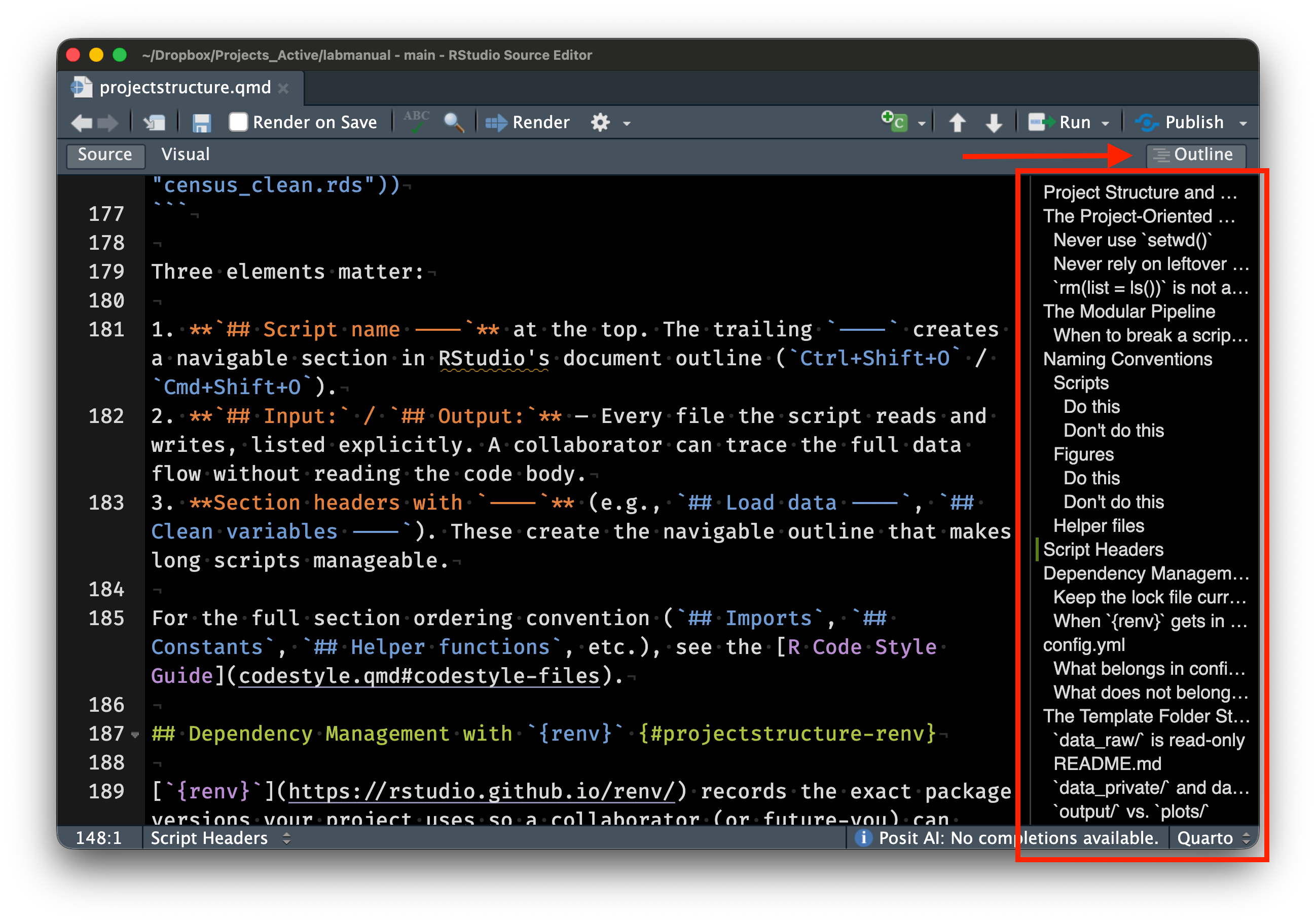
readr::write_rds(census_clean, here::here("data", "census_clean.rds"))

Three elements matter:

1. ## Script name ---- at the top. The trailing ---- creates a navigable section in RStudio’s document outline (Ctrl+Shift+O / Cmd+Shift+O).
2. ## Input: / ## Output: — Every file the script reads and writes, listed explicitly. A collaborator can trace the full data flow without reading the code body.
3. Section headers with ---- (e.g., ## Load data ----, ## Clean variables ----). These create the navigable outline that makes long scripts manageable.

Use the “Outline” button in RStudio to see your section headers!

For the full section ordering convention (## Imports, ## Constants, ## Helper functions, etc.), see the R Code Style Guide.

Dependency Management with {renv}

{renv} records the exact package versions your project uses so a collaborator (or future-you) can reproduce the environment. Three commands cover 90% of usage:

## Initialize renv for a new project (run once)
renv::init()

## After installing or updating packages, record the current state
renv::snapshot()

## Restore the recorded state on a new machine
renv::restore()

The renv.lock file is the machine-readable record of your dependencies — commit it to Git. The renv/library/ folder is .gitignored because it contains the actual installed packages (large, platform-specific).

ImportantKeep the lock file current

If you install a new package (e.g., install.packages("survival")), run renv::snapshot() before committing. A stale renv.lock defeats the purpose — a collaborator who runs renv::restore() will get the wrong package versions.

When {renv} gets in the way

{renv} occasionally causes friction: slow installs, conflicts with system libraries, or packages that fail to compile. Here’s what I’ve found helps:

• renv::deactivate() temporarily turns off renv for the session if you need to debug a package installation issue. renv::activate() brings it back.
• renv::repair() re-links packages that got corrupted (e.g., after an R version upgrade).
• {renv} shares a global package cache across projects, so the same version of {dplyr} isn’t duplicated on disk ten times. Disk usage is not as bad as it looks.
• For projects that use only base R and a few stable {tidyverse} packages, {renv} may be overkill. Use your judgment — the goal is reproducibility, not ceremony. If you skip {renv}, at minimum include a sessionInfo() call at the end of your main analysis script or save the output of sessionInfo() to a text file in the project root so a collaborator can see what versions you used.

config.yml

Project-level parameters live in config.yml. Date ranges, core counts, (low risk) file paths, analysis flags — all go in one place rather than scattered across scripts. Read them with the {config} package:

library(config)
cfg <- config::get()

start_year <- cfg$start_year
n_cores    <- cfg$n_cores

Centralizing parameters means you can change a date range or toggle a sensitivity analysis by editing one file, instead of hunting through every script.

What belongs in config.yml

Parameter type	Example	Why centralize
Date ranges	start_year: 2010	Used in multiple scripts for filtering and labeling
Parallelization	n_cores: 4	Varies by machine; easy to override
Analysis flags	run_sensitivity: true	Toggle expensive steps during development
Sample sizes	n_bootstraps: 1000	Used in analysis and reporting

What does not belong in config.yml

Secrets (API keys, credentials, proprietary column names of high risk data) go in code/secrets.R. Parameters that are truly specific to a single script and never referenced elsewhere can stay in that script’s ## Constants section.

The Template Folder Structure

.
├── README.md        # Project overview, data sources, how to run
├── code/            # All scripts, numbered for execution order
│   ├── utils.R      # Shared helper functions
│   └── secrets.R    # API keys, server paths (gitignored)
├── config.yml       # Project parameters
├── data/            # Processed, analysis-ready data (shareable)
├── data_private/    # Restricted-access data (gitignored)
├── data_raw/        # Original source data (read-only)
├── lit/             # Background reading and key references (gitignored)
├── manuscript/      # Drafts, submission files, Google Doc links (gitignored)
├── output/          # Underlying data for figures
├── plots/           # Publication figures (PDF + JPG at ≥600 dpi)
├── qmd/             # Quarto documents for tables
└── *.Rproj          # RStudio project file

data_raw/ is read-only

Raw source data goes in data_raw/ and is never modified by hand or by script. If you download census estimates from the Bureau’s web portal, the downloaded file goes here unchanged. When your cleaning script reads it and produces an analysis-ready version, the output goes in data/.

This separation means you can rerun the entire pipeline from scratch. If data_raw/ has been hand-edited, you can’t distinguish your modifications from the original source — and neither can a reviewer.

README.md

Every project gets a README.md at the root. It’s the first thing a collaborator (or future-you) reads. At minimum, include:

• Project title and one-sentence description
• Data sources and how to obtain them
• How to run the analysis (e.g., “run scripts in code/ in numbered order”)
• Any non-obvious dependencies or setup steps

You don’t need to write a novel. A README that answers “what is this and how do I run it” is enough. See READMEs from these examples of research projects that used this same structure.

data_private/ and data governance

Restricted-access data (IRB-governed, DUA-protected) goes in data_private/. Everything in this folder is .gitignored except the README. The README should include information such as:

• IRB and DUA numbers
• Expiration and data destruction dates
• Storage location (e.g., Stanford Nero, GCP bucket)
• Who has access
• Rules around sharing summary statistics

Fill these in at project start. Your future self will thank you when the DUA renewal comes around.

It is critical that data that cannot be shared is only ever stored in data_private/. This is a safeguard to stop us from accidentally putting sensitive data on to Github since it is .gitignored by default. For example, recently, highly-sensitive UK Biobank data was accidentally leaked to Github by researchers who were careless who should have known better.

output/ vs. plots/

Many journals require the numerical data behind each figure. Other researchers and journalists often ask for it too. plots/ holds the rendered figures (PDF for journals, JPG at ≥600 dpi for presentations), and output/ holds the numerical representation of these figures in CSV files.

Typically, all three files (PDF, JPG, and CSV) will be saved in the same script.

qmd/ for tables

Tables in manuscripts should never be entered by hand. Quarto documents in qmd/ generate tables programmatically from the data in data/. When data or analyses change, re-rendering the Quarto document updates the table automatically.

Git Practices

What to commit

• All code (code/), config files (config.yml), Quarto documents (qmd/), and the renv.lock file.
• Processed data in data/ if small enough (under ~50 MB per file). The template’s pre-commit hook warns on files exceeding 50 MB.
• Raw data in data_raw/ if small and publicly available. If large, .gitignore it and document the download instructions in data_raw/README.md.

What not to commit

• Private data (data_private/ — already gitignored).
• Secrets (code/secrets.R — already gitignored).
• {renv} libraries (renv/library/ — already gitignored).
• Quarto build artifacts (.quarto/, *_files/ — already gitignored).
• Manuscripts and drafts (manuscript/ — already gitignored).
• Background reading PDFs (lit/ — already gitignored; most are copyrighted).

.gitignore

The template .gitignore is extensive. It excludes private data, secrets, renv internals, Quarto artifacts, large binary formats, OS junk files, and Office temporaries. Add project-specific entries as needed, but rarely remove existing ones.

One Last Thing

The underlying principle behind all of this is simple — your project should not depend on your personal setup. Jenny Bryan calls this the distinction between workflow (your editor, your desktop, your file paths) and product (the code, data, and outputs that others see). Everything in this appendix — here::here(), {renv}, config.yml, the folder structure — exists to keep your workflow out of the product.

If any of this feels like a lot, don’t worry — the template repository handles most of it for you. Start a new project from the template, and you get 90% of this structure for free. If something doesn’t make sense, just ask.

If you actually want more detail, check out my notes and slides on The Scientific Computing Workflow.

References

• Bryan, J. (2017). “Project-oriented workflow.” tidyverse blog post.
• Bryan, J. & Hester, J. (2023). What They Forgot to Teach You About R, chapters 2–4.
• Gentzkow, M. & Shapiro, J. M. (2014). “Code and data for the social sciences: A practitioner’s guide.”
• Marwick, B., Boettiger, C., & Mullen, L. (2018). “Packaging data analytical work reproducibly using R (and friends).” The American Statistician, 72(1), 80–88. DOI: 10.1080/00031305.2017.1375986
• Noble, W. S. (2009). “A quick guide to organizing computational biology projects.” PLOS Computational Biology, 5(7), e1000424. DOI: 10.1371/journal.pcbi.1000424
• Sandve, G. K. et al. (2013). “Ten simple rules for reproducible computational research.” PLOS Computational Biology, 9(10), e1003285. DOI: 10.1371/journal.pcbi.1003285
• Wilson, G. et al. (2017). “Good enough practices in scientific computing.” PLOS Computational Biology, 13(6), e1005510. DOI: 10.1371/journal.pcbi.1005510

---

1. here::here() walks up the directory tree looking for certain sentinel files (.Rproj, .here, .git). The .Rproj file in our template is what anchors it. If you work outside of RStudio (e.g., from a terminal, VS Code, or Positron), the .here file or .git folder serves the same purpose. If {here} ever resolves to the wrong root, run here::dr_here() to see exactly which sentinel file it found and where.